Article information

J Health Info Stat. 2023;48(4):291-305

Publication date (electronic) : 2023 November 30

doi : https://doi.org/10.21032/jhis.2023.48.4.291

Jinheum Kim^,

Professor, Department of Applied Statistics, University of Suwon, Hwaseong, Korea

김진흠^,

수원대학교 데이터과학부 교수

Corresponding author: Jinheum Kim. 17 Wauan-gil, Bongdam-eup, Hwaseong 18323, Korea
E-mail: jkimdt65@gmail.com

*This work was supported by the National Research Foundation of Korea (NRF) grant funded by the Korea government (MSIT) (No. RS-2023-00239958).

No potential conflict of interest relevant to this article was reported.

Received 2023 August 23; Revised 2023 September 25; Accepted 2023 November 30.

Trans Abstract

서 론

생존시간은 연구시작 시점부터 관심 있는 이벤트(예: 사망, 재발 등)의 발생 시점까지의 시간으로 정의한다. 생존자료분석에서는 생존시간에 영향을 미치는 위험인자를 찾기 위해 콕스(Cox) 비례위험모형을 널리 사용하고 있다[1,2]. 그러나 대부분의 종단 연구에서는 환자가 방문할 때마다 관심 있는 이벤트의 발생 여부뿐만 아니라 위험인자를 관측한다. 따라서 시간에 따라 변하는 위험인자가 있다면 위험인자의 기저 값과 함께 주기적으로 관측된 값을 모형에 포함할 수 있는데 이와 같은 모형을 확장 콕스(extended Cox) 모형이라고 한다[3]. 다만 이 모형은 위험비(hazards ratio)가 시간에 따라 변할 수 있기 때문에 더 이상 비례위험 가정을 만족하지 못할 수도 있다. 한편 확장 콕스 모형에서는 위험인자의 값이 연속적으로 변해도 이산적으로 근사하는 방법을 사용하기 때문에 다소 편향된 추론이 될 수 있다[4]. 따라서 위험인자의 값이 연속적으로 변할 뿐만 아니라 측정 오차를 포함하고 있으면 위험인자의 측정값보다는 평균값으로 대체하는 모형을 생각할 수 있는데 이와 같은 모형을 소위 결합 모형(joint model, JM)이라고 한다[5]. 이때 종단 위험인자에 대한 모형으로는 선형혼합모형이 널리 사용하고 있다.

2절에서는 본 논문에서 사용할 자료를 소개하고, 3절에서는 결합 모형 중에서 가장 널리 사용되는 현재 값 모형을 소개한다. 4절에서는 현재 값 모형을 여러 가지 유형의 자료로 확장하고, 5절에서는 모형 진단을 위한 여러 가지 잔차를 소개한다. 6절에서는 추정 모형의 응용으로 이벤트의 발생 확률과 종단 위험인자의 값을 예측하는 방법을 소개하고, 종단 위험인자가 환자들을 두 그룹(고위험과 저위험)으로 얼마나 잘 구분하는지를 평가할 수 있는 지수 등을 소개한다. 마지막으로 7절에서는 본 연구의 내용을 간략히 요약하고 본 논문의 제한점을 제시하고자 한다.

자료 소개

본 논문에서 사용하고자 하는 자료는 원발성 담낭 간경변증(primary biliary cirrhosis, PBC)을 가진 환자들을 대상으로 1974년부터 1984년까지 미국 메이오 클리닉(Mayo Clinic)에서 임상시험을 수행한 결과이다[6]. 디-페니실라민(D-penicillamine, DPCA)이 PBC 환자들의 생존시간을 향상시키는지 알아보기 위해 연구에 참여한 312명 중에서 임의추출한 158명에게는 DPCA을 처방하고 나머지 154명에게는 위약을 처방한 뒤 등록 시점부터 사망이나 간이식, 종료 시점(1986년 7월)까지의 시간(단위: 년)과 발생한 이벤트의 유형을 기록하였다. 125명이 사망했고, 19명이 간이식을 받았으며, 나머지 168명은 중도 탈락(lost to follow-up)하거나 중도절단되었다. 위험인자는 성별, 연령뿐만 아니라 혈청 내 빌리루빈(serBilir), 혈관 기형 여부(spider), 간비대 여부(hepatomegaly) 등이다. 이 자료는 JM 패키지[7]에서 얻을 수 있다.

Figure 1은 치료 방법(DPCA 대 위약)에 따라 생존함수의 카플란-마이어(Kaplan-Meier) 추정량[8]과 위험집합의 크기를 나타낸 그림이며, 이에 대한 R 코드는 다음과 같다.

Figure 1.

Kalan-Meier estimates of the survival function and the number of risk set at the selected times by drug for the PBC data. PBC, primary biliary cirrhosis.

로그-순위검정 결과 유의수준 5%에서 치료 방법 간에 생존함수가 다르다고 할 수 없었다(p =0.99).

종단 생존시간 자료의 결합 모형

공변량은 외적 공변량과 내적 공변량으로 나누어진다. 외적 공변량은 다시 성별 등과 같이 시간에 따라 변하지 않는 공변량과 시간에 따라 변하는 공변량으로 나누어진다. 특히 후자는 관심 있는 이벤트의 발생에는 영향을 미치지만 이벤트의 발생으로 인해 영향을 받지 않으므로 이벤트의 발생 이후에도 관측이 가능한 공변량이다. 내적 공변량이란 환자가 위험집합(risk set)에 있는 동안에만 관측이 가능한 공변량을 말한다[9]. PBC 자료에서 성별, 등록 시 연령, 치료 방법 등은 시간에 따라 변하지 않으므로 외적 공변량이고, serBilir, spider, hepatomegaly 등과 같은 바이오마커(biomarkers)들은 내적 공변량이다. 외적 공변량이 이벤트의 발생에 미치는 영향을 알아보려면 확장 콕스 모형을 사용하면 된다[3]. 다만 내적 공변량은 소위 “ last value carried for-ward”라는 원칙에 따라 인접한 관측 시점들 사이 구간에서는 공변량의 값이 변하지 않는다고 가정한다. 따라서 내적 공변량을 가진 확장 콕스 모형의 통계적 추론은 편향된 결론을 내릴 수 있다[4].

본 절에서는 내적 공변량이 생존시간에 미치는 영향을 알아보기 위해 널리 사용되고 있는 결합 모형을 소개하고자 한다. 결합 모형이란 생존시간 자료에 대한 모형(이하, 생존 모형)과 내적 공변량처럼 반복 측정된 종단 자료에 대한 모형(이하, 종단 모형)을 결합한 모형을 말한다.

첨자 i(i=1,2,…,n)와j(j=1,2,…,n_i) 는 각각 개체와 개체 내 관측 번호를 나타내고,T* 는 이벤트 발생 시간,C 는 중도절단 시간이라 고 하자. 본 논문에서 다룰 종단 생존시간 자료는 다음과 같다.

여기서 T_i=min(T^*_i,C_i),δ_i = I(T^*_i≤C_i) 이고 y_i = (y_i(t_i1),y_i(t_i2),…,Y_i(t_in1))' 는n_i × 1 종단 자료 값 벡터이다. 또한Y_i(t) 는 t 시점에서 관측한 i-번째 개체의 종단 자료 값이다.

m_i(t)는 시점t 에서 i-번째 개체의 관측할 수 없는 참(true) 종단 값이라고 하고,m~i(t)={mi(s),0≤s<t} 는t 바로 직전 시점까지 종단 자료 값의 프로세스라고 하자. 먼저 생존 모형을 다음과 같이 정의하자.

여기서 h₀(t) 는 기저위험함수이고 W_i 는 외적 공변량 벡터이다. h₀(t) 는 와이블분포나 조각지수분포, B-스플라인 등처럼 모수적으로 가정 하거나 비모수적으로 가정할 수 있다. 한편 종단 모형을 다음과 같이 정의하자.

여기서 x_i(t)는 고정 효과에 대한 디자인 벡터이고, z_i(t) 는 (1,t)',(1,t,t²)' 등처럼 랜덤 효과에 대한 디자인 벡터이다. 랜덤 효과 벡터 b_i ∼ N(0,D) 라고 가정하고, 측정 오차는 ε_i(t) ∼ N (0,σ²) 이라고 가정하자. b_i와 ε_i(t) 는 서로 독립이라고 가정하자.

모형 (1)과 (2)에서 추정해야 할 모수 벡터는 θ = ( θ^'_t, θ^'_y, θ^'_b)이다. 여기서 θ_t = (γ^',α, θ^'_h0)' 은 생존 모형에 관한 모수 벡터이고, θ_y = (β^',σ²)' 은 종단 모형에 관한 모수 벡터, θ_b = vec(D) 는 랜덤 효과에 관한 모수 벡터이다. 여기서 θ_h0 은 기저위험함수에 대응하는 모수 벡터를 의미한다. 특히 α 는 바이오마커와 이벤트 발생 위험 간의 연관성을 나타내는 모수이고 본 논문에서 관심 있는 가설은 H₀:α = 0 이다.

결합 모형에 대한 우도 함수를 정의하기 위해 다음 세 가지를 가정하자.

특히 (A2)는 이벤트 발생 이후 결측 되는 종단 자료 값에 무관하게 추론이 가능하도록 해준다. 따라서 i-번째 개체의 (관측 자료) 우도 함수는 다음과 같이 표현된다.

θ에 대한 최대우도추정량은 EM[10] 알고리즘을 써서 로그-우도함수

를 최대로 하는 θ로 정의된다. 그러나 EM 알고리즘은 추정량의 수렴 속도가 선형적이라는 단점이 있다[11]. (관찰 자료) 스코어 벡터는 (완전 자료) 스코어 벡터의 랜덤 효과에 대한 사후 분포의 기댓값으로 표현되는데 이를 구체적으로 표현하면 다음과 같다[5].

여기서

이다. θ 의 최대우도추정량을 θ^ 라고 하면θ^ 의 공분산 행렬은 식 (4)를 써서 다음과 같이 추정된다.

여기서 I(θ^)=−∂∂θ′S(θ)|(θ=θ^) 는 관찰 자료 정보 행렬이다. 한편 콕스 모형이나 확장 콕스 모형은 부분 우도(partial likelihood)로부터 회귀 모수를 추정하므로 기저위험함수를 명시하지 않아도 회귀 모수에 대한 추론이 가능하다[3]. 그러나 결합 모형에서는 부분 우도를 사용하지 못하고 완전 우도(full likelihood)를 사용하므로 누적 기저위험함수 즉H0(t)=∫0th0(s)ds 가 서로 다른 이벤트 발생 시점에서만 변하는 계단 함수라는 가정하에서 추정해야 한다[12,13]. 그러나 n이 크면 θ_h0 의 차원이 매우 커서 식 (5)의 계산이 어려우므로 θ_h0 의 추정량을 프로파일 추정량θ^h0 으로 대체한 후 θ_h0 를 제외한 나머지 모수의 추정량의 표준오차만 추정하는 방법을 사용한다[12].θ^h0 의 표준오차는 부스트랩(bootstrap)을 사용하여 추정할 수 있지만 결합 모형에서는 시간이 많이 요구되는 단점이 있다[12].

PBC 자료에서 질병 악화의 지시자(indicator)로 serBilir를 고려하고자 한다. 기저 시점, 6개월 후, 1년 후, 그 이후부터는 매년 한 번씩 serBilir를 관측하여 312명의 환자로부터 총 1,945개의 측정값을 얻었다. 환자 1인당 평균 6.2번 반복 측정한 셈이다. Figure 2는 특정 환자들의 serBilir 값(동그라미)과 평활 값(파란색: 위약, 오렌지색: DPCA)을 나타낸 그림이며, 이에 대한 R 코드는 다음과 같다.

Figure 2.

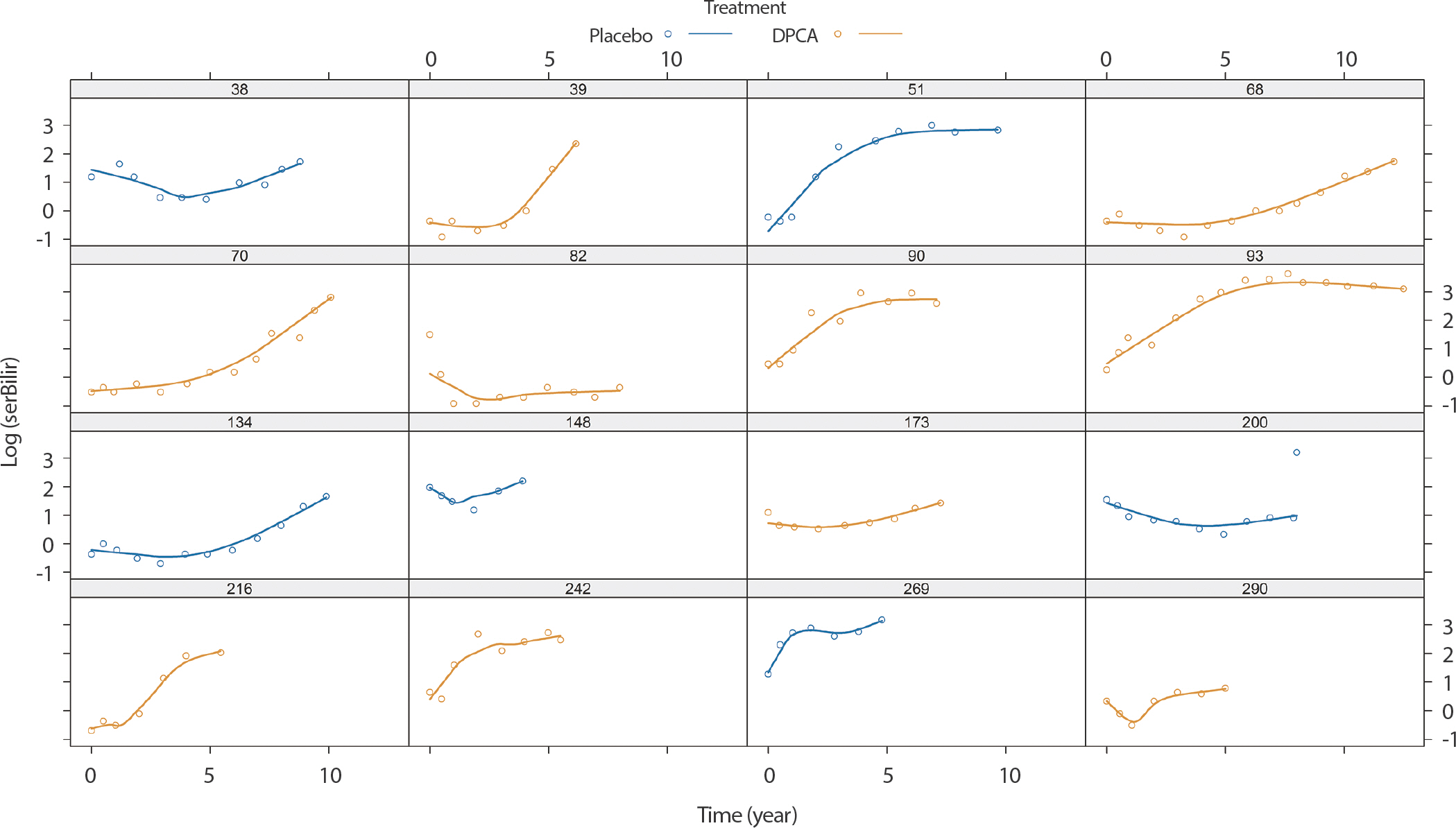
Subject-specific longitudinal profiles for sixteen patients from PBC data. PBC, primary biliary cirrhosis.

serBilir의 평활 곡선으로 볼 때 serBilir는 시간(단위: 년)에 따라 비선형적으로 변하고 치료 방법에 따라 변하는 경향이 있다고 할 수 있다. 따라서 다음과 같은 m_i(t)를 가진 종단 모형을 가정하고자 한다.

또한 생존 모형은 다음과 같이 가정하고자 한다.

Table 1은 기저위험함수에 따라 모형 (6)과 (7)의 결합 모형에 대한 회귀 모수와 연관성 모수의 추정값과 표준오차를 정리한 것이다. 한편 serBilir를 외적 공변량으로 정의하면 모형 (7)은 다음과 같이 표현된다.

Table 1.

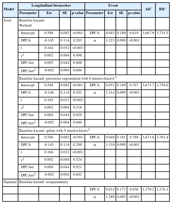
Estimates of regression parameters and their standard errors for longitudinal biomarker and/or event parts in the joint models with three different baseline hazard functions and in the extended Cox model

Table 1은 확장 콕스 모형 (8)에 대한 회귀 모수의 추정값과 표준오차도 포함하고 있으며, 이에 대한 R 코드는 다음과 같다¹⁾

세 결합 모형에서 회귀 모수의 추론 결과는 기저위험함수에 관계없이 유사하였으며, 가장 작은 AIC [14]와 BIC [15] 값을 가진 와이블 분포 모형이 최적 모형이라고 할 수 있다. 결합 모형과 확장 콕스 모형의 생존시간에 대한 회귀 모수의 추정량을 비교하면 두드러진 차이는 없었지만 연관성 모수는 확장 콕스 모형에서 과소추정됨을 알 수 있다.

결합 모형의 확장

본 절에서는 3절에서 정의한 모형 (1)과 (2)를 확장한 모형을 소개하고자 한다.

첫째, 생존 모형 (1)은 종단 자료의 현재 값 m_i(t) 에 의존하므로 모형 (1)을 소위 “현재 값” 모형이라고 부른다. 이벤트의 발생 위험이 종단 자료의 현재 값과 변화율에 의존하는 모형(“현재 값+변화율” 모형이라고 부름)으로 확장할 수 있으며, 이 모형은 모형 (1)을 변형하여 다음과 같이 정의된다.된다.

이외에도

누적값모형:hi(t|m~i(t),wi)=h0(t)exp(γ′wi+α∫0tm(s)ds),

지연(lag)모형: hi(t∣m~i(t),wi)=h0(t)exp⁡(γ′wi+αmi(max(t−c,0)))

(단, c는 양의 상수),

상호작용모형:h1(t∣m¯1(t),w1)=h0(t)exp⁡(γ′wi1+α1 m1(t)+α2(w12×m1(t)))

공유 랜덤 효과 모형:hi(t∣m~i(t),wi)=h0(t)exp⁡(γ′wi+α′bi) 등이 있다

PBC 자료의 경우 m_i(t) 의 변화율과 누적 값은 식 (6)로부터 각각 다음과 같이 표현된다.

Table 2는 모형 (6)과 와이블 기저위험함수를 가진 모형 (7)의 결합 모형에서 모형 (7)을 상술한 모형으로 각각 확장하여 얻은 회귀 모수와 연관성 모수의 추정량과 표준오차를 정리한 것이며, 이에 대한 R 코드는 다음과 같다.²⁾

Table 2.

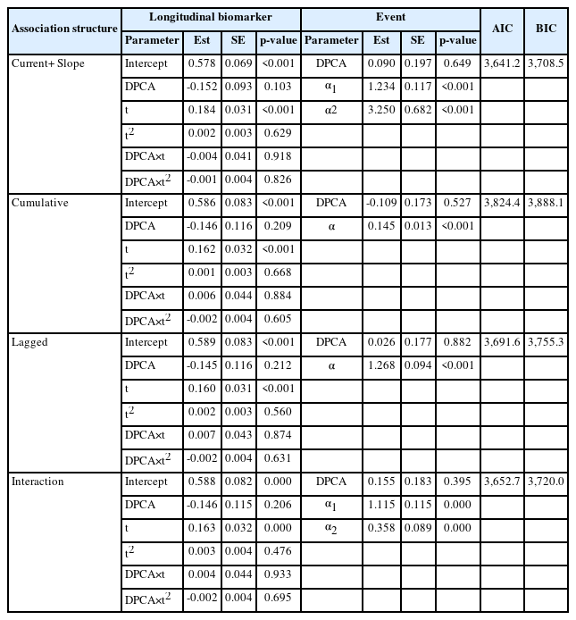
Estimates of regression parameters and their standard errors for longitudinal biomarker and event parts in the joint model under the Weibull baseline hazard function according to the association structure between the longitudinal and event outcomes

네 가지 모형 중에서는 “현재 값 + 변화율” 모형의 AIC (또는 BIC) 값이 가장 작았으며, 이 모형은 “현재 값” 모형보다도 AIC (또는 BIC) 값이 작았으며 가설H₀:α₂ = 0 에 대한 검정 결과도 통계적으로 유의하였다(p <0.001).

둘째, 생존 모형 (1)에서 외적 공변량w_i 를w_i(t) 로 대체하면 식 (3)에서hi(Ti|m~i(Ti),wi;θt) 를hi(Ti|m~i(Ti),wi;(Ti)θi) 로 대체하고, 만약w_i(t) 의 값이 구간 Ω_iq(q = 1,2,…,Q_i)에서 w_iq 로 일정하다고 하면 Si(Ti|m~i(Ti),wi;θt)를 다음과 같이 대체한다.

PBC 자료에서 시간에 따라 변하는 hepatomegaly를 모형 (7)에 hepatomegaly를 추가한 모형은 다음과 같이 정의된다.

Table 3은 모형 (6)과 스플라인 기저위험함수를 가진 모형 (9)의 결합 모형에 대한 회귀 모수와 연관성 모수의 추정량과 표준오차를 정리한 것이며, 이에 대한 R 코드는 다음과 같다.⁴⁾

Table 3.

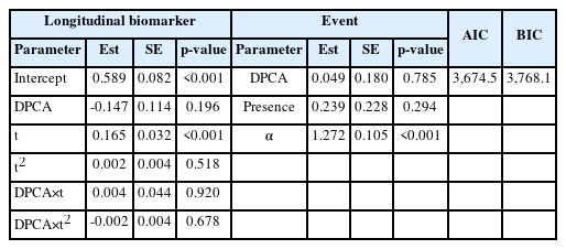
Estimates of regression parameters and their standard errors for longitudinal biomarker and event parts in the joint model with hepatomegaly (presence/absence) as an external time-dependent covariate

Hepatomegaly를 가질수록 이벤트의 발생 위험이 1.27배(95% confi-dence interval, CI: 0.81-1.99) 높지만 통계적으로 유의하지는 않았다(p =0.294).

셋째, 다기관 혹은 다국가 연구에서는 기관이나 국가마다 고유한 기저위험함수를 가정할 수 있다. 이때 기관이나 국가를 층으로 정의하고 생존 모형 (1)을 다음과 같이 확장하고자 한다.

혹은

여기서 h_0k(t) 는 k-번째 층의 기저위험함수이고, γ_k와 α_k 는 각각 k-번째 층의 회귀 모수와 연관성 모수이다. 모형 (10)과 (11)을 각각 공통 효과 모형과 층별 효과 모형이라고 부르자.

PBC 자료에서 층을 hepatomegaly의 기저 값(“ No”, “ Yes”)으로 정의하자. Table 4는 모형 (6)과 스플라인 기저위험함수를 가진 모형 (10), 모형 (6)과 스플라인 기저위험함수를 가진 모형 (11)의 결합 모형에 대한 회귀 모수와 연관성 모수의 추정량과 표준오차를 각각 정리한 것이며, 이에 대한 R 코드는 다음과 같다.⁵⁾

Table 4.

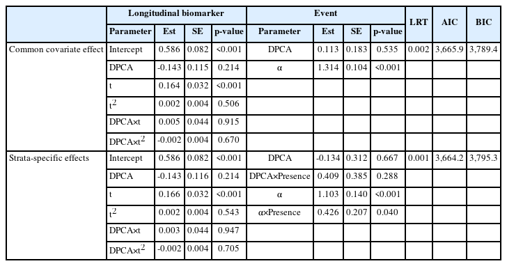
Estimates of regression parameters and their standard errors for longitudinal biomarker and event parts in the joint models stratified according to the presence or absence of hepatomegaly

Hepatomegaly 여부에 따라 기저위험함수가 통계적으로 유의하게 다르며(공통 효과 모형: p =0.002, 층별 효과 모형: p =0.001), 회귀 모수와 연관성 모수가 층별로 다른지에 대한 검정 결과는 유의수준 5%에서 통계적으로 유의하지 않았다(p =0.060). 그러나 hepatomegaly 여부에 따라 이벤트에 미치는 drug 효과는 다르지 않았지만(p =0.288), ser-Billir 효과는 유의하게 다른 것으로 나타났다(p =0.040).

넷째, 한 환자가 종단 연구 기간 동안 경험할 수 있는 이벤트가 2개 이상인 자료를 경쟁위험(competing risks) 자료라고 하는데 생존 모형 (1)을 경쟁위험 자료로 확장하고자 한다.T^*_k(k = 1,2,…,K) 는 k-번째 이벤트의 참 발생 시간이라고 하면 관측 가능한 자료의 형태는 다음과 같다.

여기서 δ_i 는 i-번째 환자의 이벤트 유형을 의미하며 중도절단된 경우에는 0으로 정의한다. k-번째 이벤트의 위험함수를 다음과 같이 정의하자. 사실 이는 층별로 기저위험함수와 회귀 모수, 연관성 모수를 고려한 모형과 동일하다.

따라서 식 (3)에서 P(T_i,δ_i|b_i; θ_t)를 다음과 같이 대체한다.

PBC 자료에서 사망과 이식을 경쟁위험 이벤트로 정의할 수 있다. Table 5는 모형 (6)과 스플라인 기저위험함수를 가진 모형 (12)의 결합 모형에 대해 이벤트의 유형별로 회귀 모수와 연관성 모수의 추정량과 표준오차를 정리한 것이며, 이에 대한 R 코드는 다음과 같다.

Table 5.

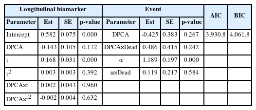
Estimates of regression parameters and their standard errors for longitudinal biomarker and event parts in the joint model with competing risks (transplanted/dead)

Drug 효과는 사망이나 이식에 통계적으로 유의하지 않았으나(사망: p =0.732, 이식: p =0.267), serBilir의 현재 값이 1 유닛 증가하면 사망의 오즈는 e^1.189+0.119 =3.70배(95% CI: 3.05-4.48)이고, 이식의 오즈는 e^1.189 =3.28배(95% CI: 2.23-4.83) 높아지는 것으로 나타났다.

다섯째, 다중(multiple) 이벤트의 다른 형태는 같은 이벤트가 반복적으로 발생하는 자료이며 이와 같은 자료를 재발 사건(recurrent event) 자료라고 부른다[16]. 에이즈 연구에서는 실제로 환자들이 사망뿐만 아니라 종단 연구 기간 동안 감염성 질병이 반복적으로 발생할 수도 있다. 에이즈 연구에서 CD4 세포 수가 적을수록 감염성 질병의 발생 횟수는 늘어나고, 또한 CD4 세포 수의 감소와 감염성 질병의 빈번한 발생은 사망의 위험을 증가시키므로 CD4 세포 수와 감염성 질병 발생, 사망을 동시에 고려하는 결합 모형이 요구된다. 따라서 반복 자료에 대한 모형을 추가하고 모형 (1)을 다음과 같이 확장하고자 한다. U_ik(k = 1,2,…,K_i)와 d_ik는 각각 i-번째 환자의 k-번째 재발 시간과 재발 여부라고 하자.

여기서 r_i(t)는 i-번째 환자의 재발 사건의 강도(intensity)이고, r₀(t)는 재발 사건의 기저강도이다. log⁡vi∼N(0,σv2) 은 랜덤 효과이며 프레일티(frailty)라고 부른다. α_r 와α_h 는 각각 종단 자료 값이 재발 강도 및 이벤트의 발생 위험과 연관된 정도를 나타내는 모수이고, 는 재발 강도가 이벤트의 발생 위험과 얼마나 강하게 연관되어 있는지를 나타내는 모수이다. 3절에서 정의한 모수 θ 를 위 모형에 맞춰 업데이트하고, 가정 (A1)을 다음과 같이 수정하자.

여기서 U_i = (U_i1,U_i2,…,U_iKi)'이고 d_i = (d_i1,d_i2,…,d_iKi)이다. 또한 다음 가정 (A4)를 추가하자.

따라서 관찰 자료에 대한 우도 함수는 3절과 유사한 방법으로 유도할 수 있다.

여섯째, 바이오마커가 두 개 이상인 자료를 분석할 수 있도록 모형 (2)를 다음과 같이 확장하고자 한다[17]. i-번째 개체의 q-번째 (q = 1,2,…, Q)종단 변수에 대한 랜덤 효과 b_iq가 주어졌을 때, t 시점에서 i-번째 개체의 q-번째 종단 자료 값 y_iq(t)에 대한 참 모형을 다음과 같이 가정하자.

여기서 x_iq(t) 와z_iq(t) 는 q-번째 종단 자료의 고정 효과와 랜덤 효과에 대한 디자인 벡터이다. 랜덤 효과 벡터b_iq ∼ N(0,D_q) 라고 가정하고, 측정 오차는ϵiq(t)∼N(0,σq2) 이라고 가정하자.b_iq 와 ∈_iq(t) 는 서로 독립이라고 가정하자. 3절에서 정의한 모수 θ를 위 모형에 맞춰 업데이트하고, 가정 (A2)를 다음과 같이 확장하자.

여기서 yi=(yi1′,yi2′,...,yiQ′),yiq=(yiq1,yiq2,...,yiqni)′,bi=(bi1,bi2,...,biQ)′∼N(0,D) 이다. 또한 Q개의 종단 자료에 맞춰 생존 모형 (1)은 다음과 같이 표현된다.

여기서 m~iq(t)={miq(s),0≤s<t} 이다. 따라서 관찰 자료에 대한 우도 함수는 3절과 유사한 방법으로 유도할 수 있다.

모형 진단

결합 모형에서 잔차는 종단 모형에 대한 잔차와 생존 모형에 대한 잔차로 구분된다. 종단 모형에 대한 잔차는 환자-중심(patient-specific) 잔차와 주변(marginal) 잔차로 나누어진다. 전자는 측정 오차에 대한 동질성 및 정규성 가정을 검정하는 데 사용하고, 후자는 고정 효과의 구조 및 환자 내 공분산 구조에 대한 가정을 검정하는 데 사용한다. 한편 생존 모형에 대한 잔차는 마팅게일(martingale) 잔차와 콕스-스닐(Cox-Snell) [18] 잔차가 있으며, 전자는m_i(t) 의 함수 꼴에 대한 가정을 검정하는 데 사용하고, 후자는 모형의 적합성을 검정하는 데 사용한다.

Figure 3은 모형 (6)과 와이블 기저위험함수를 가진 모형 (7)의 결합 모형에 대한 환자-중심 잔차와 주변 잔차, 마팅게일 잔차, 콕스-스닐 잔차를 그린 그림이며, 이에 대한 R 코드는 다음과 같다.

Figure 3.

Subject-specific standardized residuals versus subject—specific fitted values (A), marginal standardized residuals versus marginal fitted values (B), martingale residuals versus subject-specific fitted values (C) of the log of serum bilirubin, and the Kaplan-Meier estimates of the survival function of the Cox-Snell residuals (red line: the survival function of the unit exponential distribution) (D) for the PBC data. PBC, primary biliary cirrhosis.

환자-중심 잔차나 주변 잔차에서 전반적인 추세선(평활 값: 빨간색)이 0으로부터 벗어나지 않았지만 ±2를 벗어나는 잔차는 다수 관측된다. 마팅게일 잔차의 추세선(평활 값: 빨간색)은 0에 가까웠지만 종단 자료 값이 크면 약간 벗어나는 경향이 있었고, 콕스-스닐 잔차(실선)의 생존 함수 추정량(파선: 95% CI)은 참조선(평균이 1인 지수분포: 빨간색)과 거의 같았다.

이벤트 확률 및 종단 자료 값의 예측

본 절에서는 추정된 모형을 사용하여 한 환자의 이벤트 발생 확률과 종단 자료 값을 동적으로 예측하고자 하며, 바이오마커가 환자들을 고위험 환자와 저위험 환자로 얼마나 잘 구분하는지를 평가할 수 있는 동적 ROC와 AUC 및 구분 지수(discrimination index)를 소개하고자 한다.

첫째, 새로운 환자 ℓ이t(>0) 시점까지 생존해 있다고 할 때u(> t) 시점 이후에 이벤트가 발생할 다음과 같은 확률을 예측하고자 한다.

여기서 Y~ℓ(t)={yℓ(s);0≤s<t} 이고, θ^* 는 θ의 참값이다. 식 (13)은 근사 베이지안 방법[19]에 의해 다음과 같이 표현된다.

식 (14)로부터 몬테칼로(Monte Carlo) 방법을 사용하여πℓ(u|t) 를 추정하는 절차는 다음과 같다.

(Sl)θ(s)∼N(θ^,va^r⁡(θ^))를 생성한다.

(S2)bℓ(s)∼{bℓ|Tℓ∗>t,y~ℓ(t);θ(s)} 를 생성한다.

(S3)πℓ(s)(u|t)=Sℓ(u|m~ℓ(u),bℓ(s);θ(s))Sℓ(t|m~ℓ(t),bℓ(s);θ(s)) 을 계산한다.

(S4) (S1)-(S3)을 S(s = 1,2,…,S) 번 반복한다.

따라서 πℓ(u|t) 를π^ℓ(u|t)=median{πℓ(s)(u|t),s=1,2,...,S} 혹은 π^ℓ(u|t)=1S∑s=1sπℓ(s)(u|t) 로 추정한다.

Figure 4는 모형 (6)과 와이블 기저위험함수를 가진 모형 (7)의 결합 모형에 대해 id=2인 환자의 각 t=0, 1, 4.9, 6.9년에서 이벤트(사망이나 이식) 발생 확률을 동적으로 예측한 그림이며, 이에 대한 R 코드는 다음과 같다.

Figure 4.

Dynamic survival probability at specified times of 0, 1, 5, and 7 (years) for patient id = 2 from the PBC data. PBC, primary biliary cirrhosis.

id=2인 환자의 serBilir 값이 세 번째 관측 이후로 눈에 띄게 증가하므로 다섯 번째(Figure 4C)와 일곱 번째(Figure 4D) 관측 시점에서 구한 이벤트 발생 확률의 기울기가 급격하게 감소하고 있음을 알 수 있다.

둘째, 새로운 환자ℓ 이t(>0) 시점까지 생존해 있다고 할 때u(>t) 시점에서 종단 자료의 다음과 같은 기댓값을 예측하고자 한다.

식 (15)는 근사 베이지안 방법[19]에 의해 다음과 같이 표현된다.

식 (16)으로부터 몬테칼로 방법을 사용하여ω_ℓ(u|t) 를 추정하는 절차는π_ℓ(u|t) 를 예측하는 절차와 유사한데 (S1)과 (S2)는 동일하게 하고, (S3)만 다음과 같이 변형하면 된다.

(S3)′ωℓ(s)(u|t)=β^(s)′xℓ(u)+bℓ(s)′zℓ(u)를 계산한다.

따라서 ω_ℓ(u|t)를ω^ℓ(u|t)=median{ωℓ(s)(u|t),s=1,2,...,S} 혹은ω^ℓ(u|t)=1S∑s=1sωℓ(s)(u|t) 로 추정한다.

Figure 5는 모형 (6)과 와이블 기저위험함수를 가진 모형 (7)의 결합 모형에 대해 id=2인 환자의 종단 자료 값의 기댓값을 각 t=0, 1, 4.9, 6.9년에서 예측한 것이며, 이에 대한 R 코드는 다음과 같다.

Figure 5.

Dynamic prediction of the log of the serum bilirubin at specified times of 0, 1, 5, and 7 (years) for patient id=2 from the PBC data. PBC, primary biliary cirrhosis.

t에 관계없이 시간이 지남에 따라 예측 구간은 폭이 넓어지고 비대칭적인 형태를 보였다. 따라서 가까운 미래 시점의 종단 자료 값을 예측하는 것은 신뢰할 수 있지만 현재 시점으로부터 멀리 떨어질수록 예측의 정확도가 떨어진다고 할 수 있다.

셋째, 새로운 환자ℓ 의y~ℓ(t) 가 주어졌을 때 구간(t,t+dt] 에서 이벤트의 발생 여부는 환자의 처치 여부 결정하는 데 매우 중요하다. 먼저 바이오마커에 대한 예측 규칙을 정해야 하는데 간단하고 가장 널리 사용되는 규칙은 시점 t에서 관측한 바이오마커의 값을 사용하여 다음과 같이 정의하는 (시간-가변) 규칙이다.

규칙 (17)은 “시점 t에서 바이오마커의 수준이 c 이상이면 구간(t,t+Δdt] 에서 이벤트가 발생할 가능성이 높은 환자로 분류한다.”는 의미이다. 따라서 규칙 (17)에 맞춰 동적 민감도와 특이도를 정의하면 각각 다음과 같다[20].

민감도는 구간 (t,t+Δt]에서 이벤트가 발생할 환자를 바이오마커가 소위 시험군으로 분류할 확률을 의미하고, 특이도는(t + dt) 이후에 이벤트가 발생할 환자를 바이오마커가 소위 대조군으로 분류할 확률을 의미한다. 따라서 동적 ROC 곡선과 AUC를 정의하면 각각 다음과 같다[20].

여기서 [FPtΔt]−1(p)=infc{FPtΔt(c)≤p},cϵRy이다. 마지막으로 동적 구분 지수는 구간의 폭Δt 에만 의존하는데 정의하면 다음과 같다[21].

여기서 u(t)는 가중값을 의미하며T^* 의 주변분포로부터 다음과 같이 얻어진다.

몬테칼로 샘플을 사용하여 위에서 정의한 동적 민감도, 특이도, ROC 곡선, AUC 및 구분지수를 각각 추정할 수 있다[5].

Figure 6은 모형 (6)과 와이블 기저위험함수를 가진 모형 (7)의 결합 모형에 대해 id=313인 환자의 각 t=1, 3, 6, 9년에서 Δt=1, 2, 4년에 따라 동 적ROCtΔt 곡선을 그린 그림이다. Table 6은 Δt=1, 2, 4년에 따라 id=313인 환자의 각 t=1, 3, 6, 9년에서 동적AUCtΔt 와 동적 구분지수⁶⁾ C^Δt 를 추정한 것이다. 이에 대한 R 코드는 다음과 같다.

Figure 6.

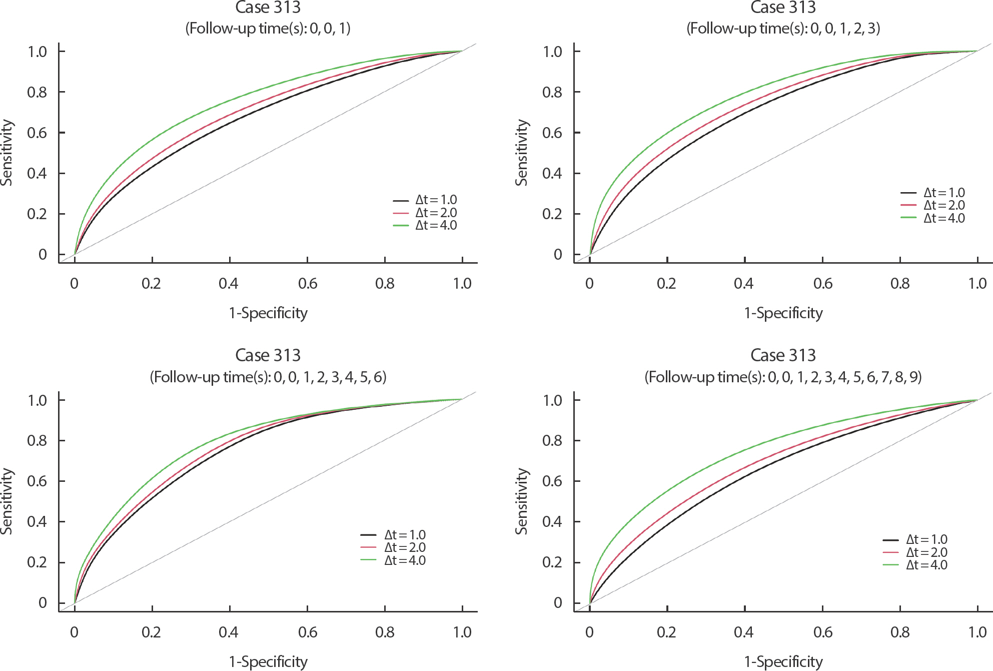
Time-dependent ROC curves at specific times of 1, 3, 6, and 9 (years) under the simple prediction rule for patient id = 313 from the PBC data. ROC, receiver operating characteristic; PBC, primary biliary cirrhosis.

Table 6.

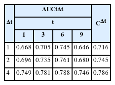
Estimated time-varying AUCs and discrimination indies of patient id=313 at four specific times with three options for Δt under the simple prediction rule

t의 값에 관계없이 Δt의 값이 증가할수록 t와t + Δt 사이에서 이벤트가 발생할 환자와t + Δt 이후에 이벤트가 발생할 환자를 구분하는 바이오마커의 예측력이 증가한다고 할 수 있다. 다만 동적 ROC와 AUC 값은 t에 의존하므로Δt 의 값을 고정했을 때t 에 따른 별다른 추이는 찾아볼 수 없었다. 한편 구분지수의 값도Δt 의 값이 증가할수록 증가함을 알 수 있다.

맺음말

본 연구에서는 종단 위험인자의 값이 연속적으로 변할 뿐만 아니라 측정 오차를 포함하고 있을 때 널리 사용되고 결합 모형을 소개하고 R 패키지 JM을 사용하여 구현하는 방법을 소개하였다. 결합 모형 중에서 가장 널리 사용되는 현재 값 모형을 소개한 후, 이 모형을 여러 가지 유형의 자료로 확장하였다. 또한 모형 진단을 위한 여러 가지 잔차를 소개하였으며, 추정 모형의 응용으로 이벤트의 발생 확률 및 종단 위험인자의 값을 예측하는 방법과 종단 위험인자가 환자들을 고위험 그룹과 저위험 그룹으로 얼마나 잘 구분하는지를 평가할 수 있는 지수 등을 각각 소개하였다.

본 연구의 제한점은, 첫째, 종단 자료의 유형(범주형, 연속형 등)에 관계없이 다룰 수 있도록 종단 모형을 일반선형혼합모형으로 확장하는 문제와, 둘째, 준경쟁위험(semi-competing risks) 자료처럼 중간 이벤트가 있는 자료를 다룰 수 있도록 생존 모형을 다중상태 자료로 확장하는 문제와, 셋째, 기저위험함수와 위험인자를 승법적인 관계로 가정했는데 가법적인 관계로 가정하는 모형이나 가속수명시간 모형으로 확장하는 문제 등을 다루지 못한 점이다.

Article information Continued